11 KiB
most of these "models" in EE are based on these DE. You'll see how important DE are in chemical, electrical, mechanical, engphys, civil (very important for civil!), (mining? idk what's in mining :D -prof) DE's are important -prof
Second order linear equations
Second order equations arise from very simple problems many engineers face, for instance a pendulum can be described by a second order equation. #second_order
$a_{2}(t)y''+a_{1}(t)y'+a_{0}(t)y=f(t)$
To motivate our interest:
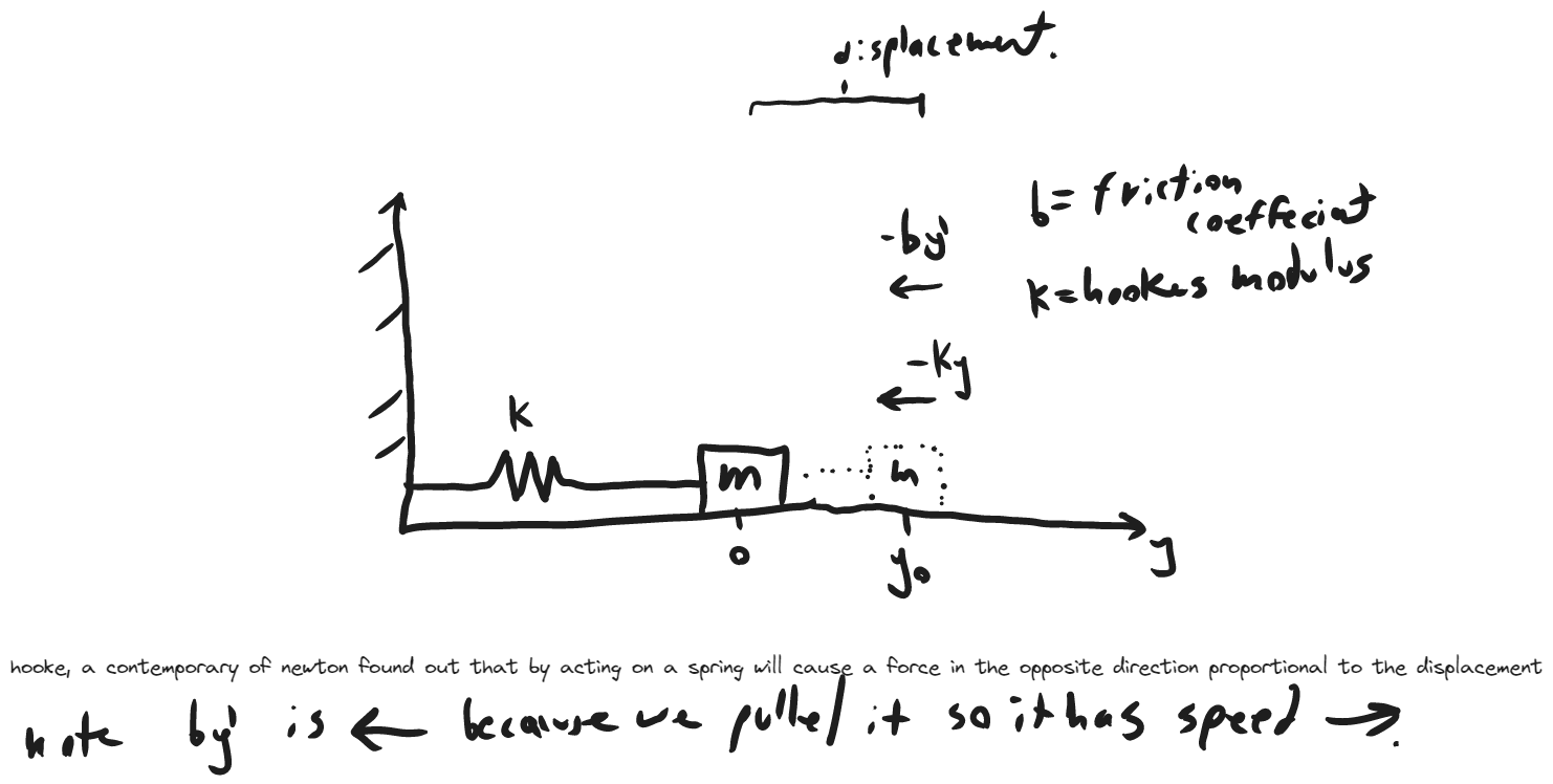
F=ma=my''
my''=-by'-ky
Look how a second order equation describes the motion of a mass-spring system!
Circuits that contains resistors, capacitors and inductors also behaves with this equation as well if you ignore the external magnetic fields around the circuit.
The equation my''+by'+ky=0 is a homogenous second order equation, because the RHS is 0. (in this case, it's full name is homogenous second order linear equation with constant coefficients.)
Similar pattern with the electrical circuit analogy. This DE ignores external forces on the mass-spring system, it only considers the friction and the spring. If we push the mass then there would be an external force and the RHS would be non zero, and the equation would be non homogenous.
It's called second order because we have second derivative in the equation.
#ex #second_order_homogenous
$y''-4y'+3y=0$
(This equation is homogenous as the RHS is equal to 0)
Imagine there's no y' (meaning no friction) you kind want the derivates to equal itself, an exponential!
We guess the solution is of the form y(t)=e^{rt}
y(t)=e^{rt}
y'=re^{rt}
y''=r^2e^{rt}
r^2e^{rt}-4re^{rt}+3e^{rt}=0 <- Our guess worked!
r^2-4r+3=0
ar^2+br+c=0
r_{1,2}=\frac{{-b\pm \sqrt{ b^2-4ac }}}{2a}
so r_{1,2}=1,3
so two possibilities of the equation:
y_{1}(t)=e^t or y_{2}(t)=e^{3t}
so the general solution is the sum of the two possibilities (But why? See principle of super position below.)
y(t)=c_{1}e^{t}+c_{2}e^{3t}and we're done.
#end of lec 5 #start of lec 6
#ex #IVP #second_order_homogenous Same equation from last lecture, but now an IVP:
y(t)=c_{1}e^{t}+c_{2}e^{3t} \quad c_{1},c_{2}\in\mathbb{R} \quad\text{let } y(0)=0,\ y'(0)=4\quad \text{ What is } c_{1}, c_{2}?Lemma: if
y(t)=c_{1}e^{t}+c_{2}e^{3t}theny'(t)=c_{1}y_{1}+c_{2}y_{2}proof: lety_{1}=e^{r_{1}t}\qquad y_{2}=e^{r_{2}t}y(t)=c_{1}e^t+c_{2}e^{3t}y'(t)=c_{1}r_{1}e^{r_{1}t}+r_{2}c_{2}e^{r_{2}t}y'(t)=c_{1}r_{1}e^{r_{1}t}+c_{2}r_{2}e^{r_{2}t}sincec_{1}r_{1}is just a product of two arbitrary constants, we can replace them with a new constant.y'(t)=c_{1}e^{r_{1}t}+c_{2}e^{r_{2}t}y'(t)=c_{1}y_{1}+c_{2}y_{2} \quad \Box
We are given y(0)=0
c_{1}e^0+c_{2}e^{3*0}=0
c_{1}+c_{2}=0
We are also given y'(0)=4
c_{1}+3c_{2}=4
Solving the linear system of equations gives: c_{1}=-2,\ c_{2}=2 which gives the solution:
y'(t)=-2e^t+2e^{3t}Principle of super position
Remember from the example above where I said the "general solution is the sum of the two possibilities"? Let's explore and see why that is:
Recap: suppose we have an equation of the form ay''+by'+cy=0
y(t)=e^{rt}
then ar^2+br+c=0
case i) r_{1},r_{2}=\frac{{-b\pm \sqrt{ b^2-4ac }}}{2a}, {r_{1}}\ne r_{2} (over damped case, there are 3 possible cases, see below.)
y_{1}(t)=e^{r_{1}t}\qquad y_{2}(t)=e^{r_{2}t}
y(t)=c_{1}e^{r_{1}t}+c_{2}e^{r_{2}t} is also a solution. But why? Principle of super position.
Principle of super position:
If y_{1}(t) solves ay''+by'+cy=f_{1}(t)
and y_{2}(t) solves ay''+by'+cy=f_{2}(t) on an interval I.
Then the following function that is a combination: y(t)=c_{1}y_{1}(t)+c_{2}y_{2}(t)
solves ay''+by'+cy=c_{1}f_{1}(t)+c_{2}f_{2}(t)
Now we prove it:
Plugging in y=c_{1}y_{1}(t)+c_{2}y_{2}(t) into ay''+by'+cy=c_{1}f_{1}(t)+c_{2}f_{2}(t) gives us:
a(c_1y_{1}''+c_{2}y_{2}'')+b(c_1y_{1}'+c_{2}y_{2}')+c(c_1y_{1}+c_{2}y_{2})=c_{1}f_{1}(t)+c_{2}f_{2}(t)
moving terms gives us: c_{1}(ay_{1}''+by_{1}'+cy_{1})+c_{2}(ay_{2}''+by_{2}'+cy_{2})=c_{1}f_{1}(t)+c_{2}f_{2}(t) \quad \Box
Okay but none of that makes sense, how do we use the proof?
Let the following:
y_{1}(t)=e^{r_{1}t} solves ay''+by'+cy=0
y_2(t)=e^{r_{2}t} solves ay''+by'+cy=0
f_{1}(t)=f_{2}(t)=0
This following can be concluded:
y(t)=c_{1}e^{r_{1}t}+c_{2}e^{r_{2}t} must solve ay''+by'+cy=0 by principle of super position.
Yay! Note this is only true when
f_{1}(t)=f_{2}(t)=0aka your RHS in the second order equation must be 0. aka the equation is homogenous.
case ii) r_{1}=r_{2}=\frac{-b}{2a} if b^2-4ac=0 (critically damped)
if we assume y_{1}=e^{r_{1}t}, y_{2}=e^{r_{1}t} like before then we get:
y(t)=c_{1}e^{r_{1}t}+c_{2}e^{r_{1}t}=ce^{r_{1}t} <- this doesn't seem like it works! We need two integration constants for a second order equation.
y_{1}(t)=e^{-bt/2a}, y_{2}(t)=te^{-bt/2a} for time being we take this as true, we can prove it later.
y(t)=c_{1}e^{-\frac{bt}{2a}}+c_{2}te^{-\frac{bt}{2a}}
we can check later at home, but also, how was the idea for this found? He will tell us later.
linear algebra 101: linear independence makes unit vectors, which forms a basis.
definition: if y_{1}, y_{2} are solutions to a(t)y''+b(t)y+c(t)=0 on some interval I_{1}
then they are called linearly independent if none of them is a constant multiple of the other.
Theorem: If y_{1}(t), y_{2}(t) are linearly independent solutions to ay''+by'+cy=0 then any other solution can be written as y(t)=c_{1}y_{1}(t)+c_{2}y_{2}(t) (due to super position)
how do we know the two solutions are linearly independent? Test for linear independence:
y_{1}, y_{2} are solutions to a(t)y''+b(t)y+c(t)y=0 on some interval I_{1}
then they are called linearly independent iff:
W(y_{1},y_{2})(t)=\det \begin{pmatrix}y_{1} & y_{2} \\y_{1}' & y_{2}'\end{pmatrix}\ne 0
case i) b^2-4ac>0 \Rightarrow r_{1}\ne r_{2}
y_{1}=e^{r_{1}t}, y_{2}=e^{r_{2}}t
W(y_{1},y_{2})=\det\begin{pmatrix}e^{r_{1}t} & e^{r_{2}t} \\r_{1}e^{r_{1}t} & r_{2}e^{r_{2}t}\end{pmatrix}
=e^{t(r_{1}+r_{2})}(r_{2}-r_{1})\ne 0 (because this can only be 0 when r_{1}= r_{2} but we know r_{1}\ne r_{2})
case ii) b^2-4ac=0\Rightarrow
r_{1}=r_{2}=-\frac{b}{2a}=r
y_{1}(t)=e^{rt}, y_{2}(t)=te^{rt}
W(y_{1},y_{2})=\det\begin{pmatrix}e^{rt} & te^{rt} \\re^{rt} & e^{rt}(1+rt)\end{pmatrix}
=e^{2rt}(1+rt)-rte^{2rt}
=e^{2rt}\ne 0
But what about case iii) ? it wasn't covered here. But now we proven that for case i and ii their two respective solutions are linearly independent and therefore we know we can safely apply the principle of super position on them and obtain their general solutions.
#ex #IVP #second_order_homogenous
y''-2y'+y=0 \qquad y(0)=1,\ y'(0)=0e^{rt}({ r^2-2r+1 })=0
(r-1)^2=0\Rightarrow r_{1}=r_{2}=1 (this is case ii, critically damped)
y(t)=c_{1}e^t+c_{2}te^t
y(0)=c_{1}=1
y(t)=e^t+c_{2}te^t
y'(0)=0
=e^0+c_{2}(0e^0+1\cdot e^0)
=1+c_{2}
\Rightarrow c_{2}=-1
y(t)=e^t-te^t#end of lecture 6 #start of lecture 7 (sept 20)
Last lecture we covered case i) and case ii).
however there's a third option:
b^2-4ac<0
Then we have complex roots:
r_{1,2}=-\frac{b}{2a}\pm\frac{i\sqrt{ 4ac-b^2 }}{2a}=\alpha\pm i\beta <- Complex conjugates. And due to fundamental theorem of algebra, there are only 2 roots in this degree 2 polynomial equation.
e^{r_{1}t}=e^{(\alpha+i\beta)t}=e^{\alpha t}+e^{i\beta t}
side note: there are no numbers that are more than two components that are "useful", even quaternions
let e^{i\beta t}=e^{i\theta}
expand into power series:
Recall from math 101:
e^x=\sum_{n=0}^\infty \frac{x^n}{n!}
=1+\frac{i\theta}{1!}+\frac{{(i\theta)^2}}{2!}+\frac{{(i\theta)^3}}{3!}+\dots
=1+\frac{i\theta}{1!}-\frac{\theta^2}{2!}-\frac{i\theta^3}{3!}+\frac{\theta^4}{4!}+\frac{i\theta^5}{5!}-\dots
=\left( 1-\frac{\theta^2}{2!}+\frac{\theta^4}{4!}-\dots \right)+i\left( \frac{\theta}{1!}-\frac{\theta^3}{3!}+\frac{\theta^5}{5!}-\dots\right)
Recall from math 101:
\cos(x)=\sum_{n=0}^\infty(-1)^n\frac{x^{2n}}{(2n)!}\quad\text{and}\quad \sin(x)=\sum_{n=0}^\infty(-1)^n\frac{x^{2n+1}}{(2n+1)!}
e^{i\theta}=\cos(\theta)+i\sin(\theta) \quad \Box We have proven the Euler formula.
we guess the solution is of the form: y(t)=e^{rt}=e^{(\alpha+i\beta)t}=e^{\alpha t}(\cos \beta t+i\sin \beta t)
Lemma: If u(t)+iv(t) solves ay''+by'+cy=0 then u(t),\ v(t) are also solutions.
Proof:
a(u+iv)''+b(u+iv)'+c(u+iv)=0
\underbrace{ { (au''+bu'+cu) } }_{ =0 }+i\underbrace{ (av''+bv'+cv) }_{ =0 }=0 <- since the RHS is zero, both the real and imaginary parts must also equal zero.
y_{1}(t)=e^{\alpha t}\cos(\beta t),\ y_{2}(t)=e^{\alpha t}\sin(\beta t)
\alpha=-\frac{b}{2a},\quad \beta={\frac{\sqrt{ 4ac-b^2 }}{2a}}
then by principle of super position:
y(t)=c_{1}y_{1}+c_{2}y_{2}
now we have to test the two solutions are linearly independent
W[y_{1},y_{2}]=\det\begin{pmatrix}y_{1} & y_{2} \\ y_{1}' & y_{2}'\end{pmatrix}\ne0
=\det \begin{pmatrix}e^{\alpha t}\cos(\beta t)& e^{\alpha t}\sin(\beta t)\\ -\beta\sin(\beta t)e^{\alpha t}+\cos(\beta t)\alpha e^{\alpha t} & \beta\cos(\beta t)e^{\alpha t}+\sin(\beta t)\alpha e^{\alpha t}\end{pmatrix}
=e^{2\alpha t}[\cos\beta t(\beta \cos(\beta t)+\alpha\sin(\beta t))-\sin \beta t(-\beta \sin(\beta t)+\alpha\cos(\beta t))]
=e^{2\alpha t}(\beta \cos^2(\beta t)+\beta \sin^2(\beta t))
=e^{2\alpha t}\beta\ne 0
Yay! We have shown the two solutions are indeed always linearly independent.
#ex #IVP #second_order_homogenous
y''-2y'+5y=0 \quad y(0)=0 \quad y'(0)=2r^2-2r+5=0<-characteristic equation
r_{1,2}=\frac{{-b\pm \sqrt{ b^2-4ac }}}{2a}
r_{1,2}={1\pm \frac{\sqrt{ -4b }}{2}}=1\pm2i
y_{1}=e^t\cos(2t) y_{2}=e^t\sin(2t)
general solution: y(t)=e^t(c_{1} \cos 2 t +c_{2}\sin 2 t)
y(0)=0=c_{1} <- this helps us calculate y' easier as we can cross out the \cos(2t) term before taking the derivative.
y'(t)=\frac{d}{dt}(e^tc_{2}\sin(2t))=e^tc_{2}2\cos(2t)+c_{2}\sin(2t)e^t
y'(0)=2=c_{2}2
therefore: c_{1}=0,\ c_{2}=1 and the solution to the IVP is:
y(t)=e^t\sin(2t)The solution has a nice graph, where if it was a circuit it would blow up, or if it was a bridge it would oscillate and eventually collapse.
In the next lecture:
something more difficult now:
ay''+by'+cy=f(t) Again, a mass-spring system without any external force.
if f(t)=0 we can find the solution easily and use superposition to get the general solution
ay''+by'+cy=0
-> general solution is y(t)=c_{1}y_{1}(t)+c_{2}y_{2}(t)
If we can find just one solution in ay''+by'+cy=f(t)
let it be y_{p}(t)
then the sum of the solutions
y(t)=c_{1}y_{1}(t)+c_{2}y_{2}(t)+y_{p}(t) must solve ay''+by'+cy=f(t)
Theorem: If a(t),\ b(t),\ c(t) are continuous on I , then IVP: a(t)y''+b(t)y'+c(t)y=f(t) ;
where y(t_{o})=y_{o} , y'(t_{o})=y_{1} has a unique solution.
we will do the proofs next class.
#end of lecture 7