#start of lec 26
We start with some thermodynamics
# Heat equation
Heat equation not only describes thermodynamics but it can also model the diffusion of gasses. It is a partial differential equation.
Strikingly, it can also model option prices in the stock market. However, using it as a strategy to make money is not so simple, because if it worked then everyone would try to use it to make money, which would cause the overall strategy to be less effective as the option prices start to get priced to accommodate for the prediction (🤯).
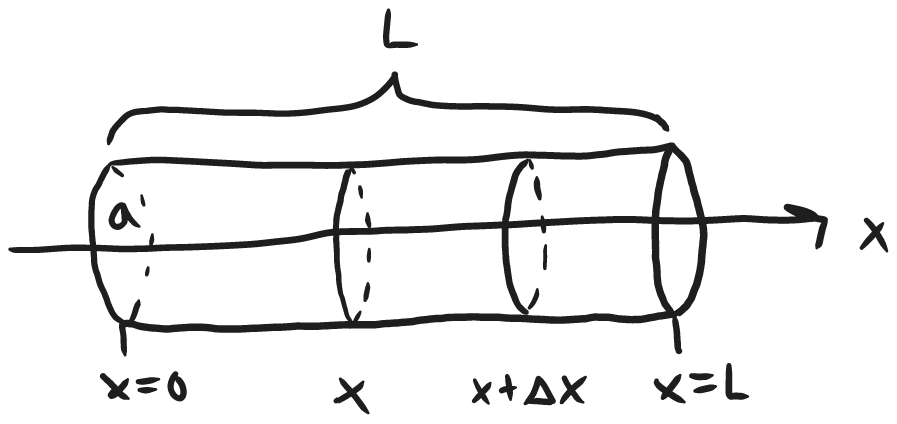
We assume that the tube is perfectly insulating along its cylindrical surface, this helps reduce the problem into a one dimensional problem. Heat can only travel inside and along the x axis.
We can express the heat along the tube as $u(t,x)$
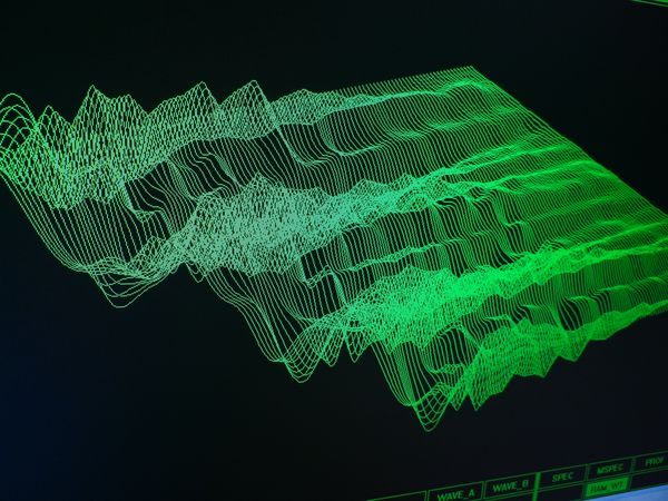
>I like to visualize $u(t,x)$ as a wavetable that smooths out as the time variable progresses. Something like this: [(image source)](https://markmoshermusic.com/2015/07/29/intro-to-loading-custom-waldorf-blofeld-wavetables/)
## Derivations (I'd skip this)
Fourier figured out that:
$\text{Heat flux} = -k(x)a\frac{\partial u}{\partial x}(t,x) \Delta t$
heat flux is in the positive $x$ direction
$k(x)$ is the thermal conductivity of the tube at point $x$
$\frac{ \partial u }{ \partial x }$ is always opposite in sign of flux (because hot flows to cold.)
$a$ is the area of the cross-section.
$=-k(x+\Delta x)a\frac{\partial u}{\partial x}(t,x+\Delta x) \Delta t$
$\Delta u=u(t+\Delta t,x)-u(t,x)$
Amount of heat to change temperature over $\Delta t$ with $\Delta u$ is $\overbrace{ C(x) }^{ \text{specific heat capacity } }\hspace{ -0.8cm}\underbrace{ \rho(x) }_{ \text{density} }\Delta u\underbrace{ a\Delta x }_{ \text{volume} }$
$C(x)\rho(x)a\Delta x(u(t+\Delta t,x)-u(t,x))=a\Delta t(k(x+\Delta x) \frac{\partial u}{\partial x}(t,x+\Delta x)-k(x) \frac{\partial u}{\partial x}(t,x))+Q(t,x)\Delta xa\Delta t$
$Q(t,x)$ is a source term, a term to model internally produced heat.
>I'm gonna be honest, I'm lost in this derivation already.
divide by $a\Delta x\Delta t$
$C(x)\rho(x)\frac{(u(t+\Delta t,x)-u(t,x))}{\Delta t}=\frac{ k(x+\Delta x) \frac{\partial u}{\partial x}(t,x+\Delta x)-k(x) \frac{\partial u}{\partial x}(t,x)}{\nabla x}+Q(t,x)$
$\lim_{ \Delta x,\Delta t \to 0 }: C(x)\rho(x)\frac{ \partial u }{ \partial t }(t,x)=\frac{ \partial }{ \partial x }\left( k(x)\frac{ \partial u }{ \partial x }(t,x) \right)+Q(t,x)$
Any differential equation, to his knowledge, is to balance some volume and to take the limit to produce a pointwise / instantaneous balance (in the form of a differential equation)
the Maxwell equations that describes magnetic and electric fields are a system of partial differential equations.
thermodynamics can be very important for electrical engineers, for instance the heat produced in a transformer, or a battery. It has applications.
## Separation of variables & Eigen value problems
#ex #SoV #evp
(This is more of a case study than an example.)
Rewrite the equation we derived by grouping the constant terms into one constant $D$ and assume for this problem that the internally generated heat is $0$ (i.e., $Q(x,t)=0$)
$\frac{ \partial u }{ \partial t }=D \frac{ \partial^2 u }{ \partial x^2 }, \quad 0\leq x\leq L, \quad t>0$
boundary conditions:
$u(t,0)=u(t,L)=0 , \quad t>0$ <- (a simple case, this is a Dirichlet boundary condition)
> Btw, Dirichlet boundary condition means the value at the two endpoints are given, A Neumann boundary condition provides information about the endpoints by giving you the derivative of the value.
$u(0,x)=f(x) , \quad 0\leq x\leq L$
These three equations form an IBVP (initial boundary value problem)
Separation of variables starts with the assumption that the solution can be written as:
$u(t,x)=T(t)X(x)$
plug into equation:
$\frac{ \partial}{ \partial t }(T(t)X(x))=D \frac{ \partial^2 }{ \partial x^2 }(T(t)X(x))$
$T'X=DTX''$
divide by $DTX$:
$\frac{T'}{DT}=\frac{X''}{X}$
recall $T$ and $X$ are single variable functions ($u(t,x)=T(t)X(x)$)
that means the left is a function of $t$ only, on the right is a function of $x$ only.
$\frac{T'}{DT}=\frac{X''}{X}=-\lambda$ where $\lambda$ is a constant
we first consider the problem:
$\frac{X''}{X}=-\lambda$
$X''+\lambda X=0$ (called an eigen value problem on a second derivative operator)
$u(t,0)=0=T(t)X(0)$
$\implies X(0)=0$
$T(t)$ cannot be the 0 term because if it was then you get $u(t,x)=T(t)X(x)=0$ for all $t$ and $x$ which can't be.
$u(t,L)=0=T(t)X(L)$
$\implies X(L)=0$
$\begin{cases}X''+\lambda X=0 \\X(0)=0 \\X(L)=0\end{cases}$ <-This is called an eigen value problem.
#end of lec 26 #start of lec 27
It's an eigen value problem because unlike before when we did second order linear equations with constant coefficients, lambda is not fixed, it can be any number.
recall in linear algebra $Ax+\lambda x=0$ where $A$ is a matrix
eigen is a Germanic word meaning intrinsic, important
We find the characteristic equations by splitting into three cases, just like we've done back in lecture 7
$X''+\lambda X=0$
case 1) $\lambda<0$
$r^2+\lambda=0 \implies r_{1,2}=\pm \sqrt{ -\lambda }$ (real solutions only since $\sqrt{ -(-) }=\sqrt{ + }$)
$X(x)=c_{1}e^{\sqrt{ -\lambda }x}+c_{2}e^{-\sqrt{ -\lambda }x}$
but we have a boundary condition:
$X(0)=0=c_{1}+c_{2}$
$c_{1}+c_{2}=0$
$X(L)=c_{1}e^{\sqrt{ -\lambda }L}+c_{2}e^{-\sqrt{ -\lambda }L}=0$
this has a unique solution, as the determinant is non-zero: $\det\left(\begin{matrix}1 & 1 \\e^{\sqrt{ -\lambda }L} & e^{-\sqrt{ -\lambda }L}\end{matrix}\right)=e^{-\sqrt{ -\lambda }L}-e^{\sqrt{ -\lambda }L}\ne 0$ (as long as $L\ne 0$, which is true since we are assuming the tube has non-zero length. Remember $\lambda\ne 0$ either since $\lambda<0$ in this case.)
the only solution is $c_{1}=0,\ c_{2}=0$
which gives $X(x)=0$ for all $x\in[0,L]$ very boring solution!
case 2) $\lambda=0$
$X''=0$
$r^2=0$
$r=0$ (repeated root)
$X(x)=c_{1}e^{0}+c_{2}0e^0=c_{1}$
$X(0)=0\implies c_{1}=0$
$X(L)=0 \implies c_{1}=0$
there are no restrictions on $c_{2}$
but our solution is $X(x)=0$ again for all $x$. This is called a trivial solution.
>alternatively, we could have found this in a different approach:
>$X''=0$
>integrate both sides twice:
>$X(x)=c_{1}x+c_{2}$
>boundary conditions:
>$X(0)=0\implies c_{2}=0$
>$X(L)=0=c_{1}L \implies c_{1}=0$
>$\implies X(x)=0$
>This method worked because the LHS is just one term of $X^n$ so we treated it as a separable equation.
We are looking for non-trival solutions. Try the last other possible case:
case 3) $\lambda>0$
$r^2+\lambda=0$
$r_{1,2}=\pm \sqrt{ -\lambda }=\pm i\sqrt{ \lambda }$
$X(x)=c_{1}\cos(\sqrt{ \lambda }x)+c_{2}\sin(\sqrt{ \lambda }x)$
boundary conditions:
$X(0)=0\implies c_{1}=0$
$X(L)=0 \implies c_{2}\sin(\sqrt{ \lambda }L)=0$
if you take $c_{2}=0$ you lose, another boring solution ($X(x)=0$).
but if $\sin(\sqrt{ \lambda }L)=0 \implies \sqrt{ \lambda }L=n\pi$
where $n=1,2,3,\dots$ notice that $n\ne 0$ because that implies $\lambda=0$ but $\lambda>0$ in case 3 so that cant be.
$\lambda_{n}=(\frac{n\pi}{L})^2$ <- These are called eigen values.
The corresponding eigen functions are:
$X_{n}(x)=c_{2}\sin(\sqrt{ \lambda_{n} }x)=c_{n}\sin\left( \frac{n\pi x}{L} \right)$
^They are the only non-trivial solutions.
lets go back to the problem and focus on $T$:
$\frac{T'}{DT}=\frac{X''}{X}=-\lambda$
$\frac{T'}{T}=-\left( \frac{n\pi}{L} \right)^2D$
this is a separable equation.
We can treat the function $T$ as a variable:
$\frac{dT}{dt} \frac{1}{T}=-\left( \frac{n\pi}{L} \right)^2D$
$\int{dT} \frac{1}{T}=\int-\left( \frac{n\pi}{L} \right)^2Ddt$
$\ln\mid T \mid=-\left( \frac{n\pi}{L} \right)^2Dt+c_{n}$
$T_{n}(t)=c_{n}e^{-(\frac{n\pi}{L})^2Dt}$
>Yes this looks illegal, but it works, you could also integrate more rigorously if you did a u-sub: $u=T(t) \quad \frac{du}{dt}=T'(t)$)
>"You might have thought you could forget the material before the midterm to make more space in your brain, your brains are a lot more emptier than mine, (class laughs) mine is filled with garbage [...] so don't forget anything you learned before the midterm!"
>"You'll see that as you continue in education, you'll see a lot of completely new things and you'll have to find shortcuts and tricks to make the content fit what you already know."
$u(t,x)=X(t)T(t)$
Okay enough with life stuff, back to mathematics:
$\implies u_{n}(t,x)=c_{n}e^{-(n\pi/L)^2Dt}\sin\left( \frac{n\pi x}{L} \right)$ $n=1,2,3,\dots$
applying superposition (sum of any solutions is also a solution):
$$u(t,x)=\sum_{n=1}^\infty c_{n}e^{-(n\pi/L)^2Dt}\sin\left( \frac{n\pi x}{L} \right)$$ ^This is the most general form of the solution.
$u(0,x)=f(x)=\sum_{n=1}^\infty c_{n}\sin\left( \frac{n\pi x}{L} \right),\ 0\leq x\leq L$ we have never seen anything like this before, an infinite number of $\sin$ terms added together, usually its polynomials that are summed.
This is when Fourier (?) steps in. He proved that you can represent various functions as a sum of sines.
fun stories about Pioncre and Cauchy Euler: Cauchy Euler was an engineer, and Pioncre had his theorem released around 2008 and it was really long, like 400 pages, he posted it online and asked if anyone wanted to prove it, after a while 4-5 or so mathematicians checked his proof and said, yep okay the proof looks correct. His theorem has a lot to do with the material world.
$f$ doesn't even have to be analytic in order for it to be expressed as a sum of sines.
Take $f(x)=\sin(x)$ and $L=\pi$ can we pick the coefficients $c_{n}$ to make the expression above true?
of course! $c_{1}=1$ and all the other coefficients equals 0.
Done with class! More history time:
Why is this important? in 1979 a team of engineers and mathematicians from a company Philips they discovered, or practically implemented that an audio signal has billions of datapoints over time if you represent it as a Fourier series, and truncate some of the coefficients we can represent many signals really well. Which condenses down the data to just a handful of coefficients
This is how filters are made too to filter out noise, just set the $c_{n}$ of the frequencies you don't want to $0$.
So Philips used math, math that is similar to what we are discussing in the lecture, to make a digital record, the first digital cd. Not only that but Fourier series are used for image and video compression as well, although they often use a sum of wavelets instead of a sum of trigonometric functions.
#end of lec 27 (Nov 10 2023)
*reading week*
#start of lec 28 (Nov 20 2023)
## Example Eigen value problem
#ex #evp
$y''-2y'+\lambda y=0 \qquad y(0)=0, \quad y'(\pi)+y(\pi)=0$
Find $\lambda$ such that the initial conditions are true.
find the characteristic polynomial:
$r^2-2r+\lambda=0$
$r_{1,2}=\frac{2\pm \sqrt{ 4-4\lambda }}{2}=1\pm \sqrt{ 1-\lambda }$
case 1: $1-\lambda>0$
$y(x)=c_{1}e^{(1+\sqrt{ 1-\lambda })x}+c_{2}e^{ (1-\sqrt{ 1-\lambda })x }$
$y(0)=0=c_{1}+c_{2}$
$y'(\pi)+y(\pi)=0$
$\implies c_{1}(1+\sqrt{ 1-\lambda })e^{(1+\sqrt{ 1-\lambda })\pi}+c_{2}(1-\sqrt{ 1-\lambda })e^{ (1-\sqrt{ 1-\lambda })\pi }+c_{1}e^{(1+\sqrt{ 1-\lambda })\pi}+c_{2}e^{ (1-\sqrt{ 1-\lambda })\pi }=0$
substitute $c_{1}=-c_{2}$
$-c_{2}(1+\sqrt{ 1-\lambda })e^{(1+\sqrt{ 1-\lambda })\pi}+c_{2}(1-\sqrt{ 1-\lambda })e^{ (1-\sqrt{ 1-\lambda })\pi }-c_{2}e^{(1+\sqrt{ 1-\lambda })\pi}+c_{2}e^{ (1-\sqrt{ 1-\lambda })\pi }=0$
$\implies c_{2}=0$
$\implies y(x)=0$ boring solution :( (also called a trivial solution)
case 2: $1-\lambda=0$
$r=r_{1,2}=1\pm \sqrt{ 0 }$ (repeated root)
$y(x)=c_{1}e^{rx}+c_{2}xe^{rx}$
$y(0)=0=c_{1}$
$y'(\pi)+y(\pi)=c_{2}(\pi e^\pi+e^\pi+\pi e^\pi)=0 \implies c_{2}=0$
(same trivial solution.)
case 3: $1-\lambda<0$
$r_{1,2}=1\pm i\sqrt{\lambda-1}$
$y(x)=e^x(c_{1}\cos(\sqrt{ \lambda-1 }x)+c_{2}\sin(\sqrt{ \lambda-1 }x))$
$y(0)=0=c_{1}$
$y(x)=c_{2}e^x\sin (\sqrt{ \lambda-1 }x)$
$y'(\pi)+y(\pi)=0=c_{2}\underbrace{ (e^\pi \sin \sqrt{ \lambda-1 }\pi+e^\pi \cos( \sqrt{ x-1 }\pi)\sqrt{ \lambda-1 }+e^\pi \sin \sqrt{ \lambda-1 }\pi) }_{ =0 }$
$$2\sin(\sqrt{ \lambda-1 }\pi)+\sqrt{ \lambda-1 }\cos(\sqrt{ \lambda-1 }\pi)=\frac{0}{e^\pi}=0$$
This is a transcendental equation, non algebraic, cannot be solved explicitly.
Btw the eigen function is $y(x)=ce^x\sin(\sqrt{\lambda-1}x)$
Only option we have is to approximate the eigen values. There are an infinite number of them.
We have to use software in order to obtain a finite number of approximations. I like software, software is good, as long as your being mindful of how you're using it. (I'm not putting quotes as I can't recall for certain what he said.)
"Engineers over design things." first they use software and add a 50%, sometimes 300% margin on it. But if your using that big of a margin I can just tell you how far you need to build your house away from the river. -Prof
Here's a plot, every crossing of red line with the $x$ axis is a solution for $\lambda$. Blue is a solution curve corresponding with $\lambda\approx8.305027$. Green shows the DE is being satisfied. And the equation on the bottom left shows the second initial condition is being met. The first condition is also met as you can see $Y(0)=0$ on the plot.
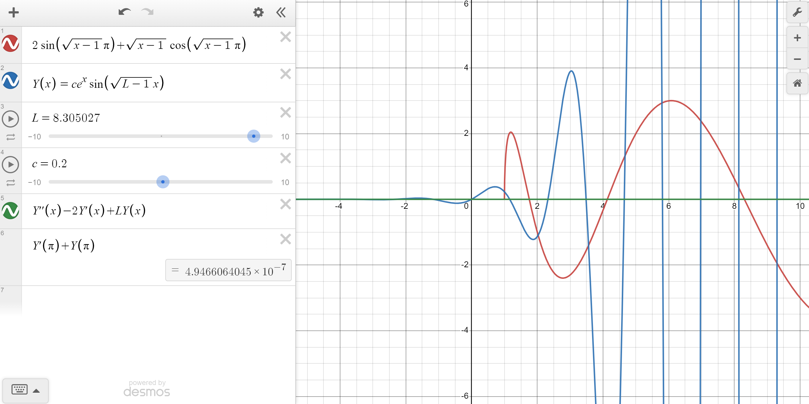
We are done.